What Does That Button Do? A Discussion on Product Manufacturing and Learning Curves

In the first blog of this series, we discussed the effects of various quantity-related inputs in a simple hardware cost estimate. This time, we will focus on a set of inputs that directly impact a specific activity in TruePlanning: Production Manufacturing. This activity will be very important for acquisition programs as it typically represents the highest cost along with non-recurring engineering.

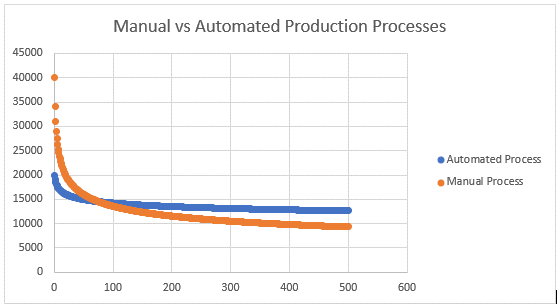
Very simply put, cost improvement curves generally depend on two factors:1. Where do you start?2. How fast do you come down the improvement curve?The “Where do you start” factor is represented by the theoretical first unit cost or T1. The “How fast do you come down the curve” factor is represented by the learning curve slope. There is a relationship between these two factors. For mature, highly automated manufacturing processes, the T1 will generally be lower and the learning curve slope will be relatively flat. Automated processes do not present as much opportunity for cost improvement or learning. For immature processes with a lot of touch labor, the T1 will generally be higher and the learning curve slope will be much steeper. Manual processes, especially new processes, present the most opportunity for learning and improvement over time. See the figure below for an example comparing manual versus automated processes.

Of course, we have all been exposed to the theory and math behind learning curves. The point of this blog is not to delve into Y=Axb. It is to discuss how key inputs in TruePlanning can be tailored to represent the environment you anticipate for your program and how those inputs affect your estimate.

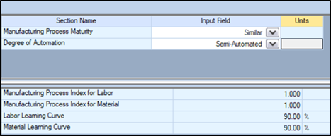
In TruePlanning, we reflect the magnitude of cost or effort for the first unit with an input called Manufacturing Process Index. It is a linear scalar to the T1 (called First Piece Cost in TruePlanning). We also reflect the steepness or shallowness of the learning curve slope with an input appropriately called Learning Curve Slope. Calculator-driven guidance within the TruePlanning Hardware Component input sheet guides the user to find suitable pairs of inputs, as shown below.

The full list of calculator results is listed below. For all possible combinations of automation and process maturity, the Manufacturing Process Index value and Learning Curve Slope are shown.

Note that TruePlanning also allows the user to set different curves and index values for labor versus material. In addition to obtaining suggested input values from the calculator, users may enter values directly on the input sheet. When no information is available, TruePlanning will internally calculate learning curves and manufacturing process index values based on the production quantity and schedule. Regardless of the method used to obtain values, the values in the model calculation can be seen on the Metrics tab. The resulting cost or effort over time can be viewed on the Results and/or Chart tabs.How do these two inputs affect your results? Recall my last blog on quantities. For a hardware component, we are estimating the cost of two phases: development and production. Within each of these phases, we have engineering, manufacturing, and tooling and test. Allow me to generalize a bit; there are always exceptions, but the following statements hold true for the majority of programs I have been involved with. In a typical weapon system acquisition program, the non-recurring engineering will generally be the biggest cost in the development phase. The recurring manufacturing will generally be the biggest cost in the production phase. And finally, production is generally more costly than development. You can see the phases and activities here:

If those generalizations hold true, then the production manufacturing activity is pretty important! It will typically represent the biggest portion of cost in an estimate. For that reason, we need to accurately represent the manufacturing environment in terms of maturity and automation. Here are three steps to achieve this:

1. Leave the inputs alone! This step seems counterintuitive but trust me. Let your schedule and production quantity phasing influence the TruePlanning internal calculation of the Manufacturing Process Index and Learning Curve Slope. If the program of record is forecasting production of 1,000 widgets in a year, an automated process is assumed. If you are building one widget every two years, a manual process is assumed. See what those internally calculated values are by viewing the Metrics tab for any hardware component.
2. Use the calculators! Once you have an idea of what TruePlanning has determined are the most appropriate input values from Step 1, you can adjust the values as necessary using the onboard calculator or ‘wizard’ on the hardware component input sheet. Using the calculator ensures the Manufacturing Process Index and Learning Curve Slope will have the right relationship between the two inputs. It will prevent you from inadvertently modeling a very high T1 with a flat learning curve slope, or a very low T1 with a steep learning curve slope (unless you really want to…).
3. Calibrate! As more information becomes available, you can calibrate the first piece or T1 cost using the Manufacturing Process Index inputs. As learning curves are negotiated or become clearer through actual / historical cost analysis, you can adjust the Learning Curve Slope inputs. Calibration will dial in perhaps the biggest portion of your overall cost estimate.

Produce activity-based estimates of cost, schedule and uncertainty using TruePlanning integrated framework with validated, predictive models for a standard, repeatable model–based cost engineering process based on the organization and technical solution being produced.

‍Learn more